Thermodynamic relations

For a general physical system there is a wide range of characteristic length and time scales, which makes numerical simulation a challenging task. As small scale physics can have large effects on the large scale dynamics of a system, an accurate description of both is required to gain understanding on more complex mechanisms occuring in such systems. Phase-field modeling allows the study of interfacial dynamics by inclusion of the mesoscale physics from a thermodynamic basis. Four common thermodynamic potentials are:

1. Internal energy \(U\) is the capacity to do work plus the capacity to release heat.

2. Helmholtz energy \(F\) is the capacity to do both mechanical and non-mechanical work (contant \(T\)).

3. Gibbs energy \(G\) is the capacity to do non-mechanical work (contant \(T\) and \(P\)).

4. Enthalpy \(H\) is the capacity to do non-mechanical work plus the capacity to release heat (contant \(P\)).

The differences between the four thermodynamic potentials are:

(17)\[\begin{split}\begin{split} d(pV) &= dH - dU = dG - dF, \\ d(TS) &= dU - dF = dH - dG \end{split}\end{split}\]

Combining the first and second laws of thermodynamics for an open PVT system lead to

(18)\[dU = T dS - PdV + \sum_{i=1}^M\mu_i dN_i, \label{eq:T1} % dU = (dU/dS)_{V,n} * dS + (dU/dV)_{S,n} * dV + (dU/dn)_{S,V} * dn\]

where the chemical potential \(\mu\) is the change of internal energy per mole of substance added to the system (at constant \(S\) and \(V\)), and \(M\) is number of phases within the system. For a two-phase system (\(M=2\)) this relation can be simplified to

(19)\[dU = T dS - PdV + \mu dC,\]

where \(C\) is a continuous phase fraction between 0 and 1. As the phase fraction is continuous, the interface \(\Gamma\) between these phases can be considered as diffuse. Nevertheless, the theoretical interface is still considered to be an infinitesimal thin boundary layer (known as the Gibbs dividing plane) and therefore sharp. This aspect is important only for curved interfaces, as curvature strongly depends on the assumed location of the interface. Eq.19 is a fundamental thermodynamic relation, and as it includes only functions of state it is true for all changes (not just reversible).

From this equation the following relations can be derived

(20)\[\begin{split}\begin{split} \left( \frac{\partial U}{\partial S} \right)_{V,C} &= T, \\ \left(\frac{\partial U}{\partial V} \right)_{S,C} &= -P, \\ \left(\frac{\partial U}{\partial C} \right)_{V,S} &= \mu. \end{split}\end{split}\]

The chemical potential term can be used to maintain a equilibrium interface profile (as done in the Cahn-Hilliard equation by the profile potential \(\omega_{p}\)). In such a case it will perform work, as it will reposition the interface. Contact line dynamics can be added in a similar way [1], which would lead to

(21)\[dU = T dS - PdV + \mu dC + \Theta d\theta,\]

with

(22)\[\begin{split}\begin{split} \left( \frac{\partial U}{\partial S} \right)_{V,C,\theta} &= T, \\ \left( \frac{\partial U}{\partial V} \right)_{S,C,\theta} &= -P, \\ \left( \frac{\partial U}{\partial C} \right)_{V,S,\theta} &= \mu, \\ \left( \frac{\partial U}{\partial \theta} \right)_{V,S,C} &= \Theta. \end{split}\end{split}\]

The last term, \(\Theta\), can be considered as a contact angle potential, which becomes zero for a certain steady state contact angle. From a thermodynamic perspective, its purpose is to decrease the free energy to its minimum state.

Important consequences from Eq.22 are that \(P\) must be independent from \(C\) and \(\theta\), \(\mu\) must be independent from the contact angle \(\theta\), and \(\Theta\) must be independent from the \(V\) and \(C\). This implies that the boundary condition for \(C\) must not affect the contact angle \(\theta\), so a neutral boundary condition is required.

Enthalpy

The enthalpy \(H\) is defined for a \(PVT\) system as

(23)\[H = U + PV.\]

Helmholtz energy

The Helmholtz (free energy) function \(F\) is defined by

(24)\[F \equiv U - TS, \label{eq:helmholtz}\]

and sets an upper limit to the non-\(PdV\) work is a process at constant temperature (isothermal) and volume (isochoric). By using T1 and helmholtz it follow for the change of Helmholtz free energy

(25)\[\begin{split}\begin{split} dF &= dU - TdS - SdT \notag \\ &= - SdT - PdV + \sum_{i=1}^{M} \mu_i dN_i. \end{split}\end{split}\]

Next one could state that \(dV=0\) since total mass is conserved, however for a two-phase system \(dV\neq0\) is possible when the enclosed mass is not conserved. Consider two phases \(\alpha\) and \(\beta\), which give the following relation for the Helmholtz free energy

(26)\[\begin{split}\begin{split} dF &= dF^{\alpha} + dF^{\beta}\\ &= - S^{\alpha}dT^{\alpha} - S^{\beta}dT^{\beta} -P^{\alpha} dV^{\alpha} -P^{\beta} dV^{\beta} + \sum_{i=1}^{M} \mu_i^{\alpha} dN_i^{\alpha} + \sum_{i=1}^{M} \mu_i^{\beta} dN_i^{\beta}. \end{split}\end{split}\]

Total mass will be conserved if

(27)\[dV = dV^{\alpha} + dV^{\beta} = 0,\]

which leads to \(dV^{\alpha} = -dV^{\beta}\). Furthermore, the following relations hold

(28)\[\begin{split}\begin{split} -S dT &= - S^{\alpha}dT^{\alpha} - S^{\beta}dT^{\beta}, \\ \sum_{i=1}^{M} \mu_i dN_i &= \sum_{i=1}^{M} \mu_i^{\alpha} dN_i^{\alpha} + \sum_{i=1}^{M} \mu_i^{\beta} dN_i^{\beta}. \end{split}\end{split}\]

If the pressure jump between the two phases is \(\Delta P = P^{\beta} - P^{\alpha}\), Eq.26 simplifies to

(29)\[dF = -S dT -\Delta P \, dV^{\beta} + \sum_{i=1}^{M} \mu_i dN_i.\]

This relation shows that the Helmholtz free energy is only idential to the chemical potential for isothermal and enclosed mass conserving flows (or for flat surfaces, in which case \(\Delta P=0\)).

Gibbs energy

The Gibbs (free energy) function \(G\) is defined by

(30)\[G \equiv F + PV = H - TS = U - TS + PV,\]

and sets an upper limit to the non-\(PdV\) work is a process between two equilibrium states at the same temperature (isothermal) and pressure (isobaric). It quantifies the energy of a system excess of its internal energy \(U\). The change of Gibbs free energy is derived from T1 and Eq.30 as

(31)\[\begin{split}\begin{split} dG &= dU - TdS - SdT + PdV + VdP \notag \\ &= - SdT + VdP + \sum_{i=1}^{M} \mu_i dN_i. \end{split}\end{split}\]

For both relations the first term on the right hand side disappears (\(dT=0\)) if the system is temperature independent.

Internal energy

As the internal energy \(U\) generally involves only differentials of extensive variables [1], application of Eq.21 assumes that the contact angle \(\theta\) is also an extensive variable\footnote{Intensive variables do not depend upon the size of the system, but only on other intensive variables or the ratio of pairs of extensive variables. Examples include the temperature, the pressure, and the chemical potential. Extensive variables scale with the size of the system. Examples include the number of particles, the volume, the energy, and the constrained and equilibrium thermodynamic potentials.}. There has been some debate if the contact angle depends on the mass of a deposited liquid or not [12].

The internal energy \(U\) is a state function, which implies that it depends only on the change between states independent of the path required to change between these states. Furthermore, the principle of minimum energy states that for a closed system (with constant external parameters and entropy), \(U\) will attain a minimum value at equilibrium [11].

This can be written as

(32)\[dU = U_{1} - U_{0} = - dW,\]

which means that the total work \(W\) done by a system in any adiabatic process is equal to the decrease in the internal energy of the system \(U_{0}-U_{1}\).

Equation of state for phase-change

Phase-change is essentially a change of the thermodynamic state of a system. Therefore, in order to model phase-change a relation between thermodynamic (state) variables like temperature, density, pressure and amount of substance must be made. If \(n\) state variables are used, only \(n-1\) can be chosen freely. The remaining variable and some additional quantities as internal energy, entropy and free energy can all be expressed as state functions of these \(n-1\) state variables. The relation between the state variables is known as the equation of state (EOS), and the best known EOS is the Van der Waals EOS [18]. The Van der Waals EOS is given by

(33)\[\left( p + a \rho^2 \right) \left(\frac{1}{\rho}-b \right) = RT,\]

where \(p\) is the pressure, \(\rho\) the density, \(R\) the universal gas constant, and \(T\) the temperature. The constants \(a\) and \(b\) depend on the substance, and modify the ideal gas law for pressure dependent intermolecular interactions (attraction and repulsion) and the volume occupied by one mole of the substance, respectively. Although this EOS is frequently used, it is well known that below the condensation point and above the saturation point, each isotherm contains an unphysical non-convex region with negative compressibility \(\textrm{d}p/\textrm{d}\rho < 0\) [16].

Here it will be shown that this unphysical behavior is directly related to the presence of interfaces, which are neglected in Eq.33.

Following [6], the Helmholtz free energy \(f\) for a Van der Waals fluid can be given as a function of the temperature \(\theta\) and density \(\rho\)

(34)\[f\left( \theta, \rho \right) = -a \rho + k \theta \ln \left( \frac{\rho}{b-\rho} \right) - c \theta \ln \left( \frac{\theta}{\theta_0} \right) - d \theta + cst.\]

Given the Helmholtz free energy, the pressure \(p\) and chemical potential \(\mu\) can be derived as functions of the temperature \(\theta\) and density \(\rho\)

(35)\[\begin{split}\begin{split} p\left( \theta, \rho \right) &= \rho^2 \frac{\partial f}{\partial \rho} = kb \frac{\rho \theta}{b-\rho} - a\rho^2,\\ \mu \left( \theta, \rho \right) &= \frac{\partial \left( \rho f \right)}{\partial \rho} = k\theta \left( \frac{b}{b-\rho} + \ln \left( \frac{\rho}{b-\rho} \right) \right) - 2a\rho. \end{split}\end{split}\]

These equations can be made dimensionless by the critical variables, which are defined as

(36)\[\begin{split}\begin{split} \theta_{c} &= \frac{8ab}{27k},\\ \rho_{c} &= \frac{b}{3}, \\ p_c &= \frac{ab^2}{27}. \end{split}\end{split}\]

This leads to the following dimensionless equations

(37)\[\begin{split}\begin{split} f\left( \theta, \rho \right) &= -3 \rho + \frac{8}{3} \theta \ln \left( \frac{\rho}{3-\rho} \right) + c \theta \left( 1 - \ln \left( \theta \right) \right), \\ p\left( \theta, \rho \right) &= \frac{8\theta\rho}{3-\rho} - 3\rho^2,\\ \mu \left( \theta, \rho \right) &= \frac{8}{3} \theta \left( \frac{3}{3-\rho} + \ln \left( \frac{\rho}{3-\rho} \right) \right) - 6 \rho. \end{split}\end{split}\]

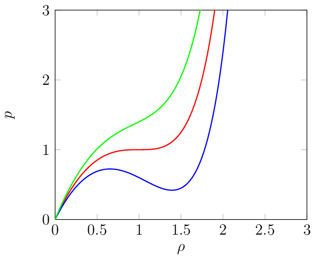
Fig. 2 Density-pressure plots for three different temperatures: below the critical temperature (blue), at the critical temperature (red), and above the critical temperature (green).

Free energy of a dividing surface

Although the Van der Waals EOS is capable of describing any phase, the free energy function as given by Eq.34 does not include interfacial effects. The free energy of a dividing surface \(\Gamma\) is given by

(38)\[f_{\Gamma} \left( A_{\Gamma} \right) = \sigma A_{\Gamma}, \label{eq:interface_free_energy_kappa}\]

where \(\sigma\) and \(A_{\Gamma}\) are the interfacial energy per unit area and the area of the interface \(\Gamma\), respectively. By definition the interface is the location with a rapid change of physical properties (like the density \(\rho\) or viscosity \(\mu\)). Therefore, the easiest method to compute the interfacial area is by something similar to

(39)\[A_{\Gamma} \sim \alpha \int_{\Omega} \left| \nabla C \right| \textrm{d}V,\]

where \(C\) is a smooth phase indicator value, and \(\alpha\) a scaling term related to the interface volume for unit area. In order to have an accurate computation of the interface area, the value of \(C\) should be constant in each phase and the interface thickness should remain constant in time. However, it is also possible to relate \(A_{\Gamma}\) with the enclosed volume \(V_{\Gamma}\) (through the first variation formula for area and volume), and write Eq.38 as a function of the volume \(V\)

(40)\[f_{\Gamma} \left( V \right) = \sigma \frac{\partial A_{\Gamma}}{\partial V_{\Gamma}} V_{\Gamma} = -\sigma \kappa_{\Gamma} H_{\Gamma} V,\]

where \(\kappa_{\Gamma}\) and \(H_{\Gamma}\) are the interface mean curvature and the Heaviside step function at the interface, respectively. After replacing the volume \(V\) by \(1/\rho\), this relation can be added to Eq.34

(41)\[\begin{split} f\left( \theta, \rho \right) &= \underbrace{-a \rho + k \theta \ln \left( \frac{\rho}{b-\rho} \right) - c \theta \ln \left( \frac{\theta}{\theta_0} \right) - d \theta}_{f_{vdw}} - \underbrace{\frac{\sigma \kappa}{\rho} H_{\Gamma}}_{f_{\Gamma}} + cst. \end{split}\]

This changes the pressure \(p\) and chemical potential \(\mu\) to

(42)\[\begin{split}\begin{split} p\left( \theta, \rho \right) &= - \left( \frac{\partial f}{\partial V} \right)_{S} = \rho^2 \left( \frac{\partial f_{vdw}}{\partial \rho} \right) - \frac{\partial f_{\Gamma}}{\partial V_{\Gamma}} \frac{\partial V_{\Gamma}}{\partial V} = kb \frac{\rho \theta}{b-\rho} - a\rho^2 + \sigma% \frac{\partial A_{\Gamma}}{\partial V_{\Gamma}} \kappa_{\Gamma} H_{\Gamma},\\ \mu \left( \theta, \rho \right) &= \left( \frac{\partial f}{\partial N} \right)_{S} = \frac{\partial \left( \rho f_{vdw} \right)}{\partial \rho} + \frac{1}{\rho} \frac{\partial f_{\Gamma}}{\partial V} = k\theta \left( \frac{b}{b-\rho} + \ln \left( \frac{\rho}{b-\rho} \right) \right) - 2a\rho. %+ \frac{\sigma \kappa_{\Gamma}}{\rho} H_{\Gamma}. \end{split}\end{split}\]

Next consider a circular liquid droplet with a dimensionless radius of \(1/4\) inside an unit square domain filled with vapor. If the droplet is at equilibrium, the densities and temperature in each phase are uniform. This implies that also the pressure and chemical potentials in each phase are uniform, and the following relations must therefore hold

(43)\[\begin{split}\begin{split} \frac{8\theta\rho_l}{3-\rho_l}-3\rho_l^2 + \sigma \kappa_{\Gamma} H_{\Gamma} &= \frac{8\theta\rho_v}{3-\rho_v}-3\rho_v^2,\\ \frac{8}{3} \theta \left( \frac{3}{3-\rho_l} + \ln \left( \frac{\rho_l}{3-\rho_l} \right) \right) - 6 \rho_l + \sigma \kappa_{\Gamma} \delta_{\Gamma} &= \frac{8}{3} \theta \left( \frac{3}{3-\rho_v} + \ln \left( \frac{\rho_v}{3-\rho_v} \right) \right) - 6 \rho_v. \end{split}\end{split}\]

These relations can be simplified to

(44)\[\begin{split}\begin{split} \sigma \kappa_{\Gamma} &= 8\theta \left( \frac{\rho_v}{3-\rho_v} - \frac{\rho_l}{3-\rho_l} \right) - 3 \left( \rho_v^2-\rho_l^2 \right),\\ &= 8 \theta \left( \frac{3(\rho_v - \rho_l)}{(3-\rho_v)(3-\rho_l)} \right) - 3 \left( \rho_v^2-\rho_l^2 \right)\\ \sigma \kappa_{\Gamma} \delta_{\Gamma} &= 8\theta \left( \frac{1}{3-\rho_v} - \frac{1}{3-\rho_l}\right) + \frac{8}{3} \theta \left( \ln \left( \frac{\rho_v}{3-\rho_v} \right) - \ln \left( \frac{\rho_l}{3-\rho_l} \right) \right) - 6 \left( \rho_v - \rho_l \right)\\ &= 8 \theta \frac{\rho_v-\rho_l}{(3-\rho_l)(3-\rho_v)} + \frac{8\theta}{3} \ln \left( \frac{\rho_v ( 3-\rho_l)}{\rho_l(3-\rho_v)} \right) - 6 \left( \rho_v - \rho_l \right). \end{split}\end{split}\]

The Heaviside function can be a smooth function given by

(45)\[H( \rho ) = \frac{\rho_v+\rho_l}{2} + \frac{\rho_l-\rho_v}{2} \tanh \left( \frac{2\rho - \left( \rho_v+\rho_l\right)}{\epsilon (\rho_l-\rho_v)} \right)\]

On the interface, where \(\delta_{\Gamma}=1\), this leads to

Assume that the dimensionless stable (equilibrium) densities are given by \(\rho_v=0.1\) and \(\rho_l=2.8\).

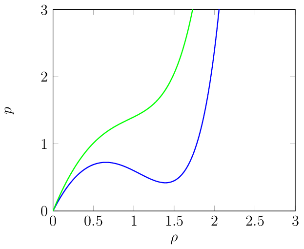
Fig. 3 Caption

For a single phase system thermodynamic equilibrium will be obtained once the pressure, temperature and chemical potential have become uniform within the whole domain. For